
Observability and monitoring of software service infrastructure is the basis for modern Site Reliability Engineering (SRE) and to successfully run and scale your IT infrastructure.
As the digital transformation of business processes and the shift towards highly dynamic cloud infrastructures keeps on accelerating, the dependency on human operation teams poses a critical bottleneck.
Especially with the grand resignation in mind and with the general lack of trained personnel the need for high-quality automation mechanisms becomes more and more important.
Automatic mechanisms such as monitoring agents and cloud integrations deliver thousands of distinct signals for millions of topological entities which are observed in real time.
Due to the advancements in network connectivity and bandwidth made in recent years, it is possible to receive a constant stream of terabytes of monitoring signal data from your production environments every day or even every minute, depending on the size of your production software system.
Besides collecting all those monitoring signals, the question arises on whether it is even possible for a human operator to derive any meaningful actions on top of those signals.
The following example should explain in detail why the observability of modern cloud infrastructures hits a hard limit for human operators and also for traditional anomaly detection mechanisms.
The scale of cloud observability
When people speak about high-cardinal data and observability signals in most cases it’s simply ignored how fast those add up when dealing with increased scale.
Let’s take a simple example where a single, traditional host is monitored. The monitoring agent sends monitoring signals for the most important aspects to observe, such as compute (CPU), memory, network and disk.
While those signals seem quite limited in number, those signals quickly add up to a much higher number if those signals are collected for various sub-dimensions of those aspects (also known as either ‘tags’ or ‘dimensions’).
Let me give you an example here.
Typically, disk utilization is not measured only on host level but much more on each disk or mount that is assigned to the host.
As hosts can have multiple disks such as ‘boot’, ‘C:’, ‘user’, … each disk signal that is collected such as ‘disk free’, ‘disk read’, ‘disk write’, ‘disk latency’, … has to be collected for each of those given disks.
This multiplies all the disk metrics by the number of disks that are present on the host.
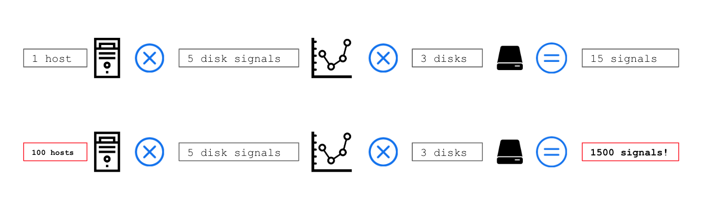
Let’s assume your host has 3 disks and you receive 5 basic disk signals, this adds up to 3 times 5 = 15 metrics per host.
What might not sound that bad, quickly adds up on a larger scale.
In case your company is monitoring 100 or more likely 1000 hosts, those 15 signals quickly will become 1500 or even 15.000 signals in large scale.
See the figure below to understand how the number of signals add up with increased scale:
In reality, each host agent collects metric signals for each running process, each disk and each network interface. This leads to hundreds of individual signals per single host, depending on the number of running processes, disks and network interfaces.
As the average number of signals collected per host is more around 50, the calculation of incoming total number of signals is closer to to the figure below:
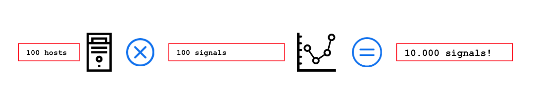
The ugly truth is that we are facing more than 5000K real time signals for 100 observed hosts, not even counting all the additional technology specific metrics, such as Tomcat, Cassandra or any other server telemetry metrics.
Looking at the current situation within companies software infrastructure, 100 observed hosts is at the very low end of the scale spectrum, where most companies continuously observe multiple thousands or even ten-thousands of hosts in parallel.
Lets see what that kind of scale means for detecting anomalies and to trigger alerts for reacting to outages.
The challenge of detecting anomalies in high cardinal data
Anomaly detection on time series metric signals is mostly based on statistics. Various different statistical methods exist that are used to identify which measurements of a given signal can be classified as being ‘normal’ versus being ‘abnormal’.
All those methods have in common that they follow the logic assumption that for any given signal most of the observed time should be in normal state, while only a small fraction of those measurements are considered as being abnormal.
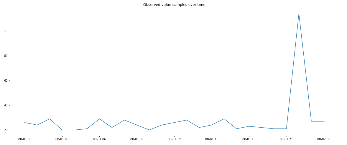
Let’s do a quick example where we measure a metric every hour for a full day. This results in 24 hourly metric samples in total.
We also assume that 99% of the time the metric is in normal state, while only 1% of the time the metric shows an abnormal level.
The below figure visualizes a time series of normal vs. abnormal measurements where the probability for a normal measurement is 99%. Just one single sample shows an abnormal level as the likelihood of 1% is relatively low compared to our 24 hour samples:
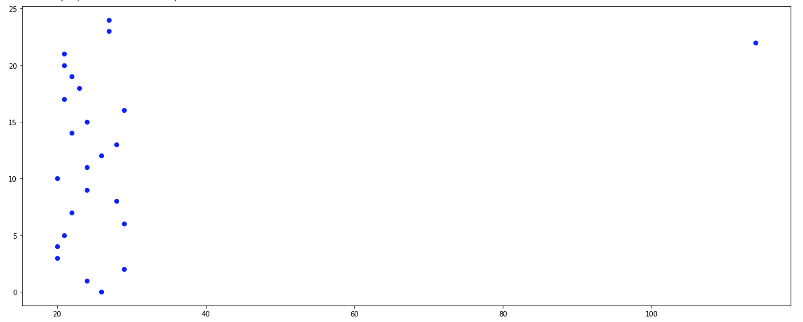
In a scatter plot visualization that outlying measurement clearly stands out compared to the large group of normal values:
As most modern real time observability platforms do not operate on hourly metric samples but much more on minute measurements, we will now do the same example with one day of minute samples but keeping the abnormal probability assumption of 1%.
A 24 hour period consists of a total of 1.440 single minute observations which multiplies the probability for abnormal observations by a factor of 60, as it shown in the chart below:

The simple truth is to understand that the number of observed samples is directly proportional with the number of abnormal situations you will detect.
While an hourly check would return around 1,68 anomalies per week with the assumption of 1% abnormality, a minute based check will yield in around 100 anomalies.
What does that mean for all my telemetry signals?
As it is mentioned in the first part of this post, today’s infrastructure and service monitoring reveals a lot of real time telemetry signals.
If we assume that a typical monitored host sends around 50 different metrics every minute, we can further assume that with a 1% abnormality probability we will end up with the following worst-case scenarios:
- 1 monitored host = 50 individual signals per minute, 1440 minutes per day results in a total of 72.000 samples per day and 504.000 samples per week.
With a 1% abnormal probability with this number of actively monitored signals you will likely end up with 5.040 identified abnormal samples per week!
- 100 monitored hosts = 100 x 50 signals x 1440 minutes = 7.200.000 samples per day and 50.400.000 samples per week, which results in 504.000 abnormal samples per week.
5.040 abnormal samples per week does not automatically mean that you would receive the same number of alerts, as anomalies are typically active and running over multiple minutes.
E.g.: if an anomaly is active for 2 hours, this would include 120 abnormal minute samples within one alert.
If we assume that all your anomalies last for 1 hour straight, you will receive 84 alerts for your continuously monitored 50 signals each single day.
The assumptions I made here of having 50 signals per host and having a 1% chance of an abnormal sample are of course artificial.
While those assumptions are very close to reality, you have to check the statistics of your own environment and how large those numbers are.
The important learning from this example should be to understand how much those numbers and their scale matter in terms of anomaly detection and alert noise.
Within the next section we will discuss possible counter measures to reduce this alert spam.
Reduce alert noise and avoid alert fatigue
It’s obvious that a high number of alerts does easily overwhelm human operators which leads to the so-called alert fatigue where alerts are no longer considered important.
A nice and well known metaphor for that situation can be found within the fable of ‘The boy who cried Wolf’. This ancient Greek fable already explained what happens when you raise too many false alarms, people don’t trust you anymore and are getting blind to the real incidents!
But now lets see what we can do to reduce the alert spam within our modern day cloud observability systems.
Choose your signals wisely
Probably the most important countermeasure is to reduce the amount of trigger signals to those that represent the most significant ones for your application.
Instead of actively checking all available telemetry signals, it’s in most cases sufficient to only trigger alerts on top of your chosen so-called ‘Golden Signals’.
It’s hard to tell which those Golden Signals are within your own service infrastructure, this could be Response time as performance signal and the error rate as the stability signal, but you might choose completely different signals entirely depending on your business model.
Adapt detection models upon criticality
While some servers or services are super critical, others are not. This should also be reflected in the sensitivity of the anomaly detection that is used to monitor their signals.
While you might want to check on a minute basis for your most critical services, a moving 15 or 30 min sliding window is more than sufficient for less critical ones.
Also differentiate between the criticality of checking the performance signal and the stability of a service. While the first one might be granted a 30 min observation period, the second one needs more sensitivity.
Check all relevant signals during root-cause analysis
Once you did select your most significant golden signals for your own infrastructure, you should apply a full signal check as root-cause analysis, to find the unknown-unknowns within all the relevant monitored signals.
As the full signal check is done after an anomaly was detected, this approach does not increase the alert spam but gives you much more insights on the detailed root-cause of the anomaly.
Modern observability platforms such as Dynatrace already offer such an automatic, AI driven root-cause detection method.
Merge single events into consistent incidents
During large-scale outages it’s inevitable that many different anomalies are detected within the affected topology. In case individual anomalies are detected, it’s important to automatically merge those into a consistent incident which share the same root cause.
As one single downstream component can cause the failure of hundreds of front end components, all anomalies along this dependency graph must be merged into a single consistent incident to avoid the sending of a storm of individual alerts.
The preferred methodology of merging those individual anomaly events is to use the discovered trace topology and dependency graph, like Dynatrace is doing.
The alternative for tools without proper topological context is to apply event pattern detection on top to rediscover topological dependencies through machine learning. The pattern detection process is imprecise and relies on a learning period, which we normally don’t have within a highly dynamic network and service environments.
Summary
The goal of this post was to show the tremendous challenges that arise with the explosion of cardinality and scale of monitoring signals in modern cloud environments.
The direct relation of monitoring scale and the number of detected anomalies leads to alert spam even if you apply the best of breed anomaly detection models.
As real time anomaly detection on millions of individual telemetry signals ultimately leads to alert spam and alert fatigue, those monitored signals must be chosen wisely.
By analyzing and selecting just a handful of relevant ‘Golden Signals’ along with some adaptations of the monitoring models, you ultimately avoid alert spam and save your Site Reliability Teams (SRE) from alert fatigue.